
In the prelude to Part I discussed the riddle of induction, and highlighted the fact that all learning requires you to make assumptions. Accepting that this is true, our first task to come up with some fairly general assumptions about data that make sense. This is where sampling theory comes in. If probability theory is the foundations upon which all statistical theory builds, sampling theory is the frame around which you can build the rest of the house. Sampling theory plays a huge role in specifying the assumptions upon which your statistical inferences rely. And in order to talk about “making inferences” the way statisticians think about it, we need to be a bit more explicit about what it is that we’re drawing inferences from (the sample) and what it is that we’re drawing inferences about (the population). In almost every situation of interest, what we have available to us as researchers is a sample of data. We might have run experiment with some number of participants; a polling company might have phoned some number of people to ask questions about voting intentions; etc. Regardless: the data set available to us is finite, and incomplete. We can’t possibly get every person in the world to do our experiment; a polling company doesn’t have the time or the money to ring up every voter in the country etc. In our earlier discussion of descriptive statistics (Chapter 5, this sample was the only thing we were interested in. Our only goal was to find ways of describing, summarising and graphing that sample. This is about to change.
Each of these defines a real group of mind-possessing entities, all of which might be of interest to me as a cognitive scientist, and it’s not at all clear which one ought to be the true population of interest. As another example, consider the Wellesley-Croker game that we discussed in the prelude. The sample here is a specific sequence of 12 wins and 0 losses for Wellesley. What is the population?
Again, it’s not obvious what the population is.

Irrespective of how I define the population, the critical point is that the sample is a subset of the population, and our goal is to use our knowledge of the sample to draw inferences about the properties of the population. The relationship between the two depends on the procedure by which the sample was selected. This procedure is referred to as a sampling method, and it is important to understand why it matters.
To keep things simple, let’s imagine that we have a bag containing 10 chips. Each chip has a unique letter printed on it, so we can distinguish between the 10 chips. The chips come in two colours, black and white. This set of chips is the population of interest, and it is depicted graphically on the left of Figure 10.1. As you can see from looking at the picture, there are 4 black chips and 6 white chips, but of course in real life we wouldn’t know that unless we looked in the bag. Now imagine you run the following “experiment”: you shake up the bag, close your eyes, and pull out 4 chips without putting any of them back into the bag. First out comes the a chip (black), then the c chip (white), then j (white) and then finally b (black). If you wanted, you could then put all the chips back in the bag and repeat the experiment, as depicted on the right hand side of Figure 10.1. Each time you get different results, but the procedure is identical in each case. The fact that the same procedure can lead to different results each time, we refer to it as a random process. 147 However, because we shook the bag before pulling any chips out, it seems reasonable to think that every chip has the same chance of being selected. A procedure in which every member of the population has the same chance of being selected is called a simple random sample. The fact that we did not put the chips back in the bag after pulling them out means that you can’t observe the same thing twice, and in such cases the observations are said to have been sampled without replacement.
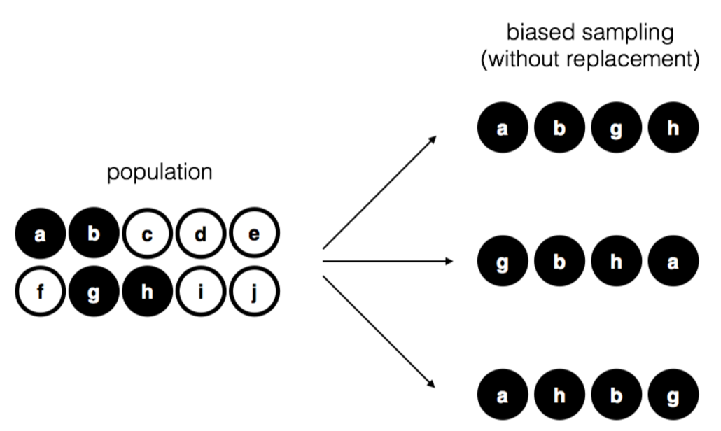
To help make sure you understand the importance of the sampling procedure, consider an alternative way in which the experiment could have been run. Suppose that my 5-year old son had opened the bag, and decided to pull out four black chips without putting any of them back in the bag. This biased sampling scheme is depicted in Figure 10.2. Now consider the evidentiary value of seeing 4 black chips and 0 white chips. Clearly, it depends on the sampling scheme, does it not? If you know that the sampling scheme is biased to select only black chips, then a sample that consists of only black chips doesn’t tell you very much about the population! For this reason, statisticians really like it when a data set can be considered a simple random sample, because it makes the data analysis much easier.

A third procedure is worth mentioning. This time around we close our eyes, shake the bag, and pull out a chip. This time, however, we record the observation and then put the chip back in the bag. Again we close our eyes, shake the bag, and pull out a chip. We then repeat this procedure until we have 4 chips. Data sets generated in this way are still simple random samples, but because we put the chips back in the bag immediately after drawing them it is referred to as a sample with replacement. The difference between this situation and the first one is that it is possible to observe the same population member multiple times, as illustrated in Figure 10.3.
In my experience, most psychology experiments tend to be sampling without replacement, because the same person is not allowed to participate in the experiment twice. However, most statistical theory is based on the assumption that the data arise from a simple random sample with replacement. In real life, this very rarely matters. If the population of interest is large (e.g., has more than 10 entities!) the difference between sampling with- and without- replacement is too small to be concerned with. The difference between simple random samples and biased samples, on the other hand, is not such an easy thing to dismiss.
As you can see from looking at the list of possible populations that I showed above, it is almost impossible to obtain a simple random sample from most populations of interest. When I run experiments, I’d consider it a minor miracle if my participants turned out to be a random sampling of the undergraduate psychology students at Adelaide university, even though this is by far the narrowest population that I might want to generalise to. A thorough discussion of other types of sampling schemes is beyond the scope of this book, but to give you a sense of what’s out there I’ll list a few of the more important ones:
Okay, so real world data collection tends not to involve nice simple random samples. Does that matter? A little thought should make it clear to you that it can matter if your data are not a simple random sample: just think about the difference between Figures 10.1 and 10.2. However, it’s not quite as bad as it sounds. Some types of biased samples are entirely unproblematic. For instance, when using a stratified sampling technique you actually know what the bias is because you created it deliberately, often to increase the effectiveness of your study, and there are statistical techniques that you can use to adjust for the biases you’ve introduced (not covered in this book!). So in those situations it’s not a problem.
More generally though, it’s important to remember that random sampling is a means to an end, not the end in itself. Let’s assume you’ve relied on a convenience sample, and as such you can assume it’s biased. A bias in your sampling method is only a problem if it causes you to draw the wrong conclusions. When viewed from that perspective, I’d argue that we don’t need the sample to be randomly generated in every respect: we only need it to be random with respect to the psychologically-relevant phenomenon of interest. Suppose I’m doing a study looking at working memory capacity. In study 1, I actually have the ability to sample randomly from all human beings currently alive, with one exception: I can only sample people born on a Monday. In study 2, I am able to sample randomly from the Australian population. I want to generalise my results to the population of all living humans. Which study is better? The answer, obviously, is study 1. Why? Because we have no reason to think that being “born on a Monday” has any interesting relationship to working memory capacity. In contrast, I can think of several reasons why “being Australian” might matter. Australia is a wealthy, industrialised country with a very well-developed education system. People growing up in that system will have had life experiences much more similar to the experiences of the people who designed the tests for working memory capacity. This shared experience might easily translate into similar beliefs about how to “take a test”, a shared assumption about how psychological experimentation works, and so on. These things might actually matter. For instance, “test taking” style might have taught the Australian participants how to direct their attention exclusively on fairly abstract test materials relative to people that haven’t grown up in a similar environment; leading to a misleading picture of what working memory capacity is.
There are two points hidden in this discussion. Firstly, when designing your own studies, it’s important to think about what population you care about, and try hard to sample in a way that is appropriate to that population. In practice, you’re usually forced to put up with a “sample of convenience” (e.g., psychology lecturers sample psychology students because that’s the least expensive way to collect data, and our coffers aren’t exactly overflowing with gold), but if so you should at least spend some time thinking about what the dangers of this practice might be.
Secondly, if you’re going to criticise someone else’s study because they’ve used a sample of convenience rather than laboriously sampling randomly from the entire human population, at least have the courtesy to offer a specific theory as to how this might have distorted the results. Remember, everyone in science is aware of this issue, and does what they can to alleviate it. Merely pointing out that “the study only included people from group BLAH” is entirely unhelpful, and borders on being insulting to the researchers, who are of course aware of the issue. They just don’t happen to be in possession of the infinite supply of time and money required to construct the perfect sample. In short, if you want to offer a responsible critique of the sampling process, then be helpful. Rehashing the blindingly obvious truisms that I’ve been rambling on about in this section isn’t helpful.
Okay. Setting aside the thorny methodological issues associated with obtaining a random sample and my rather unfortunate tendency to rant about lazy methodological criticism, let’s consider a slightly different issue. Up to this point we have been talking about populations the way a scientist might. To a psychologist, a population might be a group of people. To an ecologist, a population might be a group of bears. In most cases the populations that scientists care about are concrete things that actually exist in the real world. Statisticians, however, are a funny lot. On the one hand, they are interested in real world data and real science in the same way that scientists are. On the other hand, they also operate in the realm of pure abstraction in the way that mathematicians do. As a consequence, statistical theory tends to be a bit abstract in how a population is defined. In much the same way that psychological researchers operationalise our abstract theoretical ideas in terms of concrete measurements (Section 2.1, statisticians operationalise the concept of a “population” in terms of mathematical objects that they know how to work with. You’ve already come across these objects in Chapter 9: they’re called probability distributions.
The idea is quite simple. Let’s say we’re talking about IQ scores. To a psychologist, the population of interest is a group of actual humans who have IQ scores. A statistician “simplifies” this by operationally defining the population as the probability distribution depicted in Figure ??. IQ tests are designed so that the average IQ is 100, the standard deviation of IQ scores is 15, and the distribution of IQ scores is normal. These values are referred to as the population parameters because they are characteristics of the entire population. That is, we say that the population mean μ is 100, and the population standard deviation σ is 15.


## [1] "n= 100 mean= 99.6064025956605 sd= 16.0047604703873"
## [1] "n= 10000 mean= 100.096924966188 sd= 14.9554812898374"Now suppose I run an experiment. I select 100 people at random and administer an IQ test, giving me a simple random sample from the population. My sample would consist of a collection of numbers like this:
106 101 98 80 74 . 107 72 100
Each of these IQ scores is sampled from a normal distribution with mean 100 and standard deviation 15. So if I plot a histogram of the sample, I get something like the one shown in Figure 10.4b. As you can see, the histogram is roughly the right shape, but it’s a very crude approximation to the true population distribution shown in Figure 10.4a. When I calculate the mean of my sample, I get a number that is fairly close to the population mean 100 but not identical. In this case, it turns out that the people in my sample have a mean IQ of 98.5, and the standard deviation of their IQ scores is 15.9. These sample statistics are properties of my data set, and although they are fairly similar to the true population values, they are not the same. In general, sample statistics are the things you can calculate from your data set, and the population parameters are the things you want to learn about. Later on in this chapter I’ll talk about how you can estimate population parameters using your sample statistics (Section 10.4 and how to work out how confident you are in your estimates (Section 10.5 but before we get to that there’s a few more ideas in sampling theory that you need to know about.
This page titled 8.1: Samples, Populations and Sampling is shared under a CC BY-SA 4.0 license and was authored, remixed, and/or curated by Danielle Navarro via source content that was edited to the style and standards of the LibreTexts platform.